How Splat Forge works
A deep-dive on each pipeline stage — what's happening inside, where it spends its time, why CUDA does or doesn't apply, and how a second machine on the same LAN can help.
Where each stage actually runs
CPU on the left, GPU on the right. The further right a stage sits, the more its wall-clock time is spent inside CUDA kernels — and the more it benefits from distributing across the LAN farm onto a second card.
- 2%IngestPure CPU — EXIF parse + geodesy
- 8%Geo-alignENU similarity — pure CPU
- 12%ProjectCPU per-pixel sampling (GPU port planned)
- 14%ExportPoisson + UV unwrap + bake — mostly CPU
- 22%MapperCOLMAP IncrementalMapper + Ceres BA — CPU
- 78%ExtractSiftGPU — OpenGL FBO octaves + descriptors
- 88%MatchCUDA kernels — descriptor distance matrix
- 98%Trainsplatfacto — heavy CUDA every iter
Ingest
GPS EXIF → manifest.json + ENU origin
What it does
Walks the source-panorama directory, opens each JPEG's EXIF block, extracts GPS latitude / longitude / altitude / timestamp, writes manifest.json. The first valid GPS fix becomes the project origin and every other pano's WGS-84 coordinates are converted to a local ENU (East-North-Up, metres) frame relative to it. The actual JPEGs are not copied or modified — only metadata is written.
Architecture
Pure Python: piexif reads the EXIF block; pyproj's Transformer (EPSG:4326 → custom ENU) handles the geodesy. Origin is fixed once at start of run; every later transform is a single affine.
Compute profile
CPU only, single-threaded. Per-pano cost is dominated by JPEG header seeking on disk (~10 ms). 271 panos ingest in under 5 s on a spinning HDD, instant on NVMe.
CUDA usage
Not applicable. There's no large-scale floating-point math here — only file I/O and EXIF struct parsing.
Bottlenecks
Disk I/O. Each pano is multi-MB; we only need the first ~64 KB to read EXIF, but the OS still pays per-file open/seek/close. On slow USB this can be the difference between 5 s and 30 s.
Adding a second machine
Not worth distributing. The whole stage is so small that the ZeroMQ orchestration overhead would exceed the work. Always run ingest on the coordinator.
Project
Equirect 360 → 18 perspective views per pano
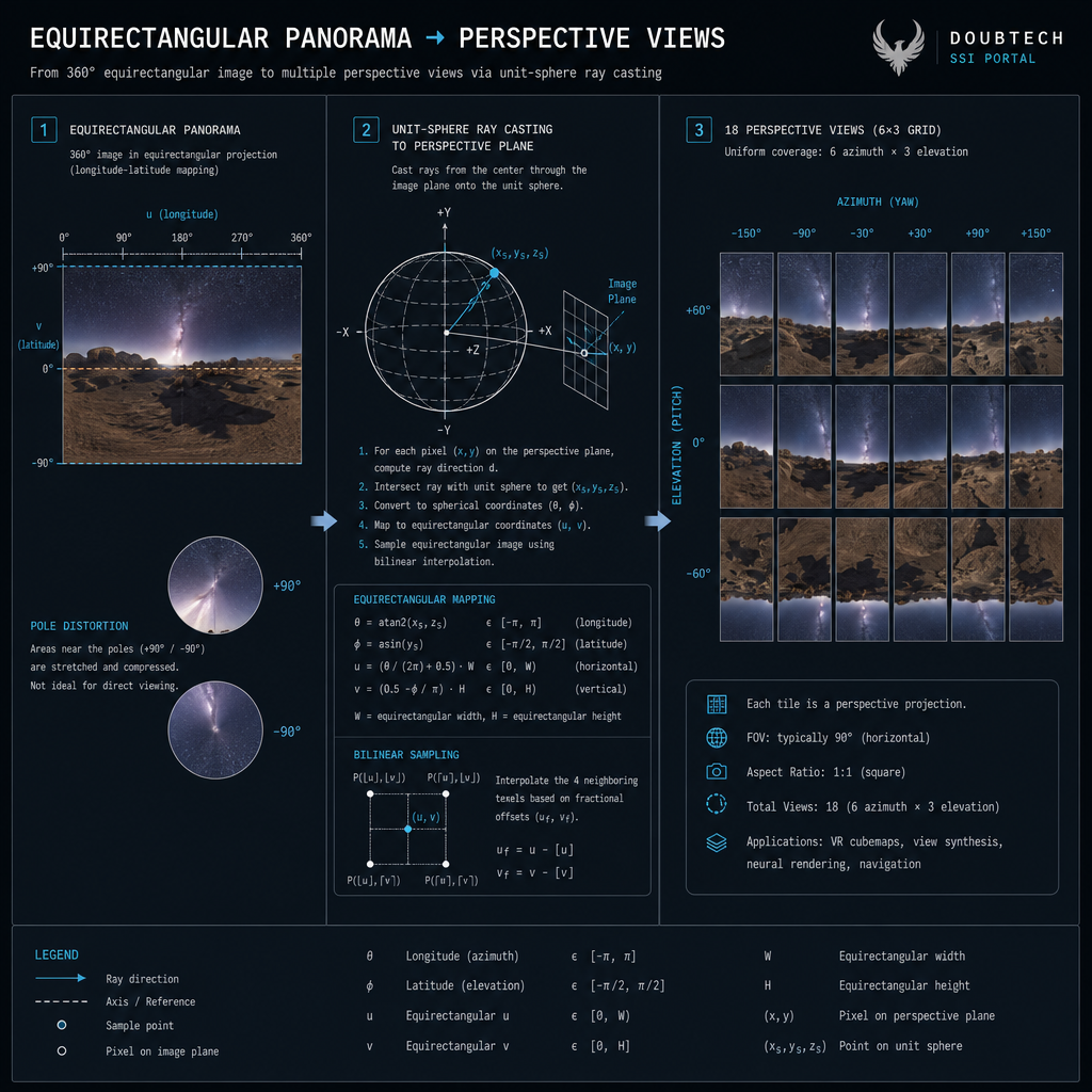
What it does
Re-renders each equirectangular panorama as conventional pinhole-camera perspective views. Default: 6 azimuths × 3 elevations = 18 views per pano at 1600×1600 px, 90° FOV. Both COLMAP's SfM and gsplat's training expect perspective input — equirect packs a full sphere into a 2:1 image with severe pole distortion that neither feature matching nor splatting handles natively.
Architecture
Per output pixel: build a unit ray from (intrinsics, rotation), intersect the unit sphere, look up that direction's bilinearly-interpolated colour in the equirect source. Wrapped in a tqdm loop with a multiprocessing pool (--workers 4) so each worker handles a disjoint subset of panos.
Compute profile
CPU-bound, embarrassingly parallel. ~3-5 s per pano per CPU core for 18 × 1600² views. With 4 workers ~25 min for 200 panos; with 24 workers the per-worker source copy starts pressuring memory.
CUDA usage
Could absolutely use CUDA but currently doesn't. Ray construction + bilinear sampling per output pixel is the textbook torch.nn.functional.grid_sample workload — 5-10× faster on a modern GPU. Roadmap item; CPU stays as a no-GPU fallback.
Bottlenecks
Pixel-write throughput. Per pano: 18 × 1600² × 3 = ~110 MB written + the equirect decompression cost. Faster storage helps marginally.
Adding a second machine
Linear speedup. Each worker can be assigned a disjoint subset of panos, render locally, post results back. Currently kept local — the LAN-farm ROI is much higher in the SfM stage where coordination matters more.
Feature extraction
SIFT keypoints per perspective image
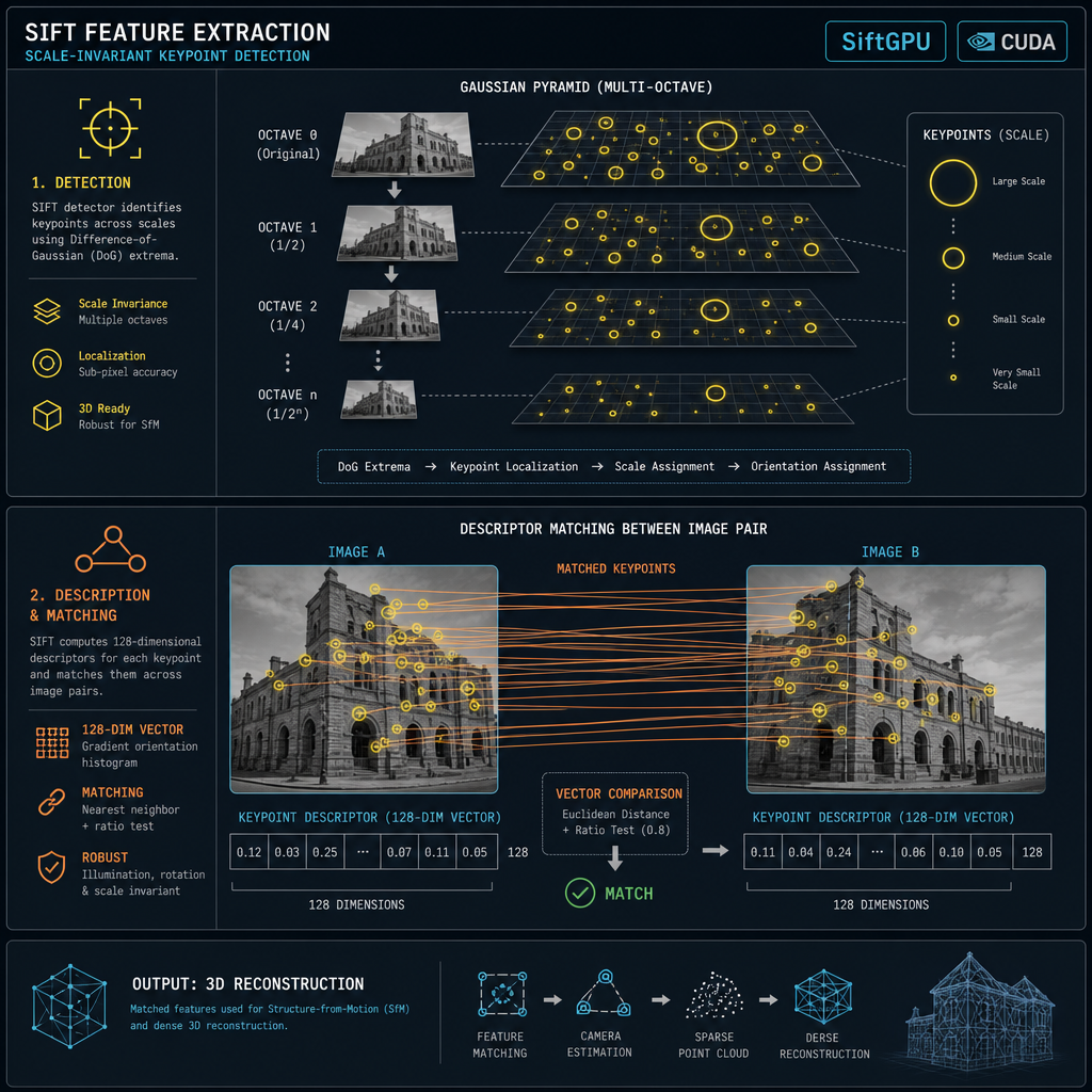
What it does
Detects ~5 000-10 000 SIFT keypoints per perspective image (a 200-pano scene with 18 views/pano = ~3 600 perspectives, ~25 M total features). Each keypoint is a sub-pixel (x, y) plus a 128-D descriptor that's invariant to scale, rotation, and modest illumination changes. Stored in a SQLite database (colmap/database.db) — typically grows to several GB on a real scene.
Architecture
COLMAP's feature_extractor with the SiftGPU backend. Octaves are built on the GPU via OpenGL FBOs; descriptor extraction runs as a fragment shader pass per keypoint location. Falls back to SIFT-CPU on hosts without a GPU.
Compute profile
GPU-bound when SiftGPU works, CPU-bound otherwise. Per-image: ~50 ms GPU vs ~500 ms CPU. A 5070 Ti chews through 3 528 perspectives in about 90 s.
CUDA usage
Indirectly. SiftGPU is OpenGL, not CUDA, but the GPU path is what matters. A future migration to CUDA-native SIFT (or a learned alternative like SuperPoint) would unlock ~3× more throughput.
Bottlenecks
GPU texture upload + DRAM bandwidth. Each perspective is loaded into a GL texture, processed, then keypoints + descriptors are read back to CPU and inserted into SQLite. SQLite insert serialisation is the secondary bottleneck.
Adding a second machine
Each worker can extract its own subset and POST keypoint records back. DB insertion is serial so the coordinator becomes the bottleneck above ~4 workers; we'd need a sharded DB or per-worker batch import to push further. Currently single-machine.
Feature matching
k-nearest GPS pairs + RANSAC verify
What it does
Decides which pairs of perspective images share enough viewpoint overlap to be worth matching, then for each chosen pair finds correspondences and runs RANSAC fundamental-matrix verification. The naive 'all-pairs' approach would be N(N-1)/2 = 6 million pairs for 3 500 perspectives — most with zero overlap. We use GPS metadata to limit each perspective's candidates to perspectives from the K=8 spatially-nearest panos. Result: ~28 K pairs instead of 6 M, two orders of magnitude faster, no real quality loss.
Architecture
A custom helper builds the GPS k-NN pair list from the manifest, writes match_pairs.txt, then COLMAP's matches_importer with --SiftMatching.use_gpu 1 consumes it: descriptor matching + RANSAC fundamental-matrix verification per pair.
Compute profile
GPU-bound on the matching kernel; CPU-bound on RANSAC and SQLite writes. Per pair: ~2-10 ms total. 28 K pairs takes ~5 minutes on a 5070 Ti.
CUDA usage
Yes. COLMAP's matching kernel uses CUDA matrix multiply for all-against-all descriptor L2 distance, with a mutual-nearest cross-check on GPU. Without CUDA the workload is ~50× slower.
Bottlenecks
Pair-list size, then GPU memory (each pair ships ~10 K × 128 floats × 2 = ~10 MB onto the GPU), then RANSAC inner loop on the CPU.
Adding a second machine
Pairs partition cleanly across workers. Each takes a slice of match_pairs.txt, matches against its own keypoint DB, and the coordinator merges the two-view geometry records. Near-linear speedup up to 4-8 workers; merge becomes the bottleneck beyond that.
Mapper (Structure-from-Motion)
3D camera poses + sparse point cloud from matches
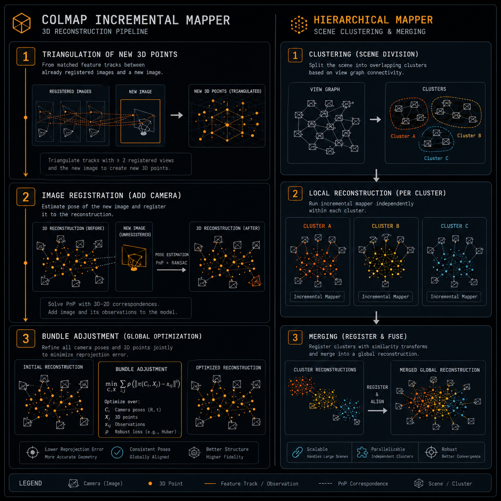
What it does
Recovers a globally consistent 3D camera-pose graph plus a sparse cloud of 3D points (typically 100 K-10 M points) from the verified two-view matches. This is the foundation everything else depends on — a bad SfM means a bad splat downstream. Three backends: colmap incremental (sequential, slow on big scenes), colmap hierarchical_mapper (default — spatial clusters mapped in parallel then merged), and glomap (single-pass global SfM — fast in theory but bottlenecked by the bundled CPU-only Ceres on Windows).
Architecture
Bundle Adjustment is the heart of every backend — a sparse non-linear least-squares problem optimising camera intrinsics + extrinsics + 3D point positions to minimise reprojection error. Solved with the Ceres library; variable count is ~10 × cameras + 3 × points = millions of unknowns.
Compute profile
CPU-bound with the Ceres builds we ship. The Schur-complement step in the inner solver is sparse Cholesky factorisation; on Windows we use Eigen's SimplicialLDLT which is single-threaded — leaving ~24 logical cores idle during the BA pass.
CUDA usage
Possible but not in our build. Ceres has cuDSS support that runs the sparse solve on GPU (~10× speedup on large scenes). Building Ceres-with-cuDSS for Windows is non-trivial. We accepted the CPU path because hierarchical mapping bounds each per-cluster BA to a small enough problem (~250 cameras) that single-threaded Cholesky finishes in minutes.
Bottlenecks
Incremental: BA frequency × per-BA cost. Hierarchical: cluster size + the merge step. GLOMAP: the single global BA at the end of the pipeline.
Adding a second machine
Best stage to farm. Each cluster from hierarchical_mapper is independent and self-contained; the data each worker needs (its image subset + the matches DB) is bounded. Splat Forge's Phase C ZeroMQ farming targets exactly this workload — coordinator splits clusters, each peer maps one in parallel, coordinator merges with `colmap model_merger`. Near-linear speedup with peer count.
Geo-alignment
Rigid transform: SfM frame → ENU world
What it does
Transforms the SfM reconstruction's arbitrary internal coordinate frame into a real-world ENU frame with metric scale and Z-up orientation. Without this the resulting splat would have unknown scale (units of arbitrary baseline length, not metres) and unknown orientation.
Architecture
COLMAP's model_aligner. Builds two N×3 matrices — SfM camera positions and ENU positions from the manifest — and runs a least-squares Procrustes fit for the (rotation, translation, scale) triple that minimises per-camera position error. We use --alignment_type=enu so the result is metric and Z-up.
Compute profile
CPU only, milliseconds. Problem size is at most a few thousand 3-vectors; the SVD-based Procrustes solve runs faster than the I/O to read the model.
CUDA usage
Not applicable. Compute is too small to saturate a GPU.
Bottlenecks
None. Effectively free.
Adding a second machine
Not worth it.
Splatfacto training
30K-iter Gaussian Splat optimisation
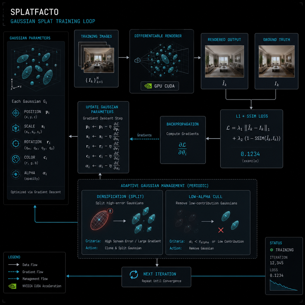
What it does
Iteratively optimises a population of 3D Gaussian ellipsoids (each with position, scale, rotation, spherical-harmonic colour, opacity) so they render the input images when projected through their camera poses. Loss is L1 + SSIM between rendered and target. Population size is dynamic — densification clones high-loss gaussians, culling removes ones with opacity below a threshold. By iter 30 K a typical scene has 1-5 M gaussians.
Architecture
nerfstudio's splatfacto config wrapping gsplat's CUDA kernels. Forward pass is a tile-based rasteriser: project gaussians into screen space, sort per tile by depth, compose with α-blending. Backward pass differentiates each step. Adam optimises positions / colours / opacities at slightly different learning rates.
Compute profile
~99 % GPU. CPU only does data loading + Python orchestration. Per-iter time on a 5070 Ti ranges from 40 ms (early, few gaussians) to 80 ms (late, many gaussians).
CUDA usage
Maximally. The custom CUDA kernels in gsplat (rasterisation, sort, α-composition, gradient kernels) ARE the workload. Without CUDA there's no useful path; CPU rasterisation would be ~1 000× slower.
Bottlenecks
GPU VRAM. As the gaussian count grows mid-run it can cross the allocator's working-set limit and crash. Splat Forge's OOM-aware wrapper auto-retries with progressively more aggressive culling — but always at native input resolution. Quality is non-negotiable: if the most aggressive cull tier still OOMs, the trainer raises and you should farm the job across the LAN rather than degrade resolution.
Adding a second machine
The big lever for VRAM-bound scenes. The Coordinator k-means-splits the scene into spatial clusters (~250 panos each) and dispatches each cluster as a WorkOffer over ZeroMQ. Each worker trains its own cluster on its own card, then results are stitched with `colmap model_merger`. A 5070 Ti + 5060 in the same room can co-train a scene that wouldn't fit either card alone. Multi-GPU on a single host (DDP-style) exists in research but isn't wired in — the LAN-farm path is the one we ship.
Export
Splat .ply / mesh.{glb,obj,fbx} / texture / KEX
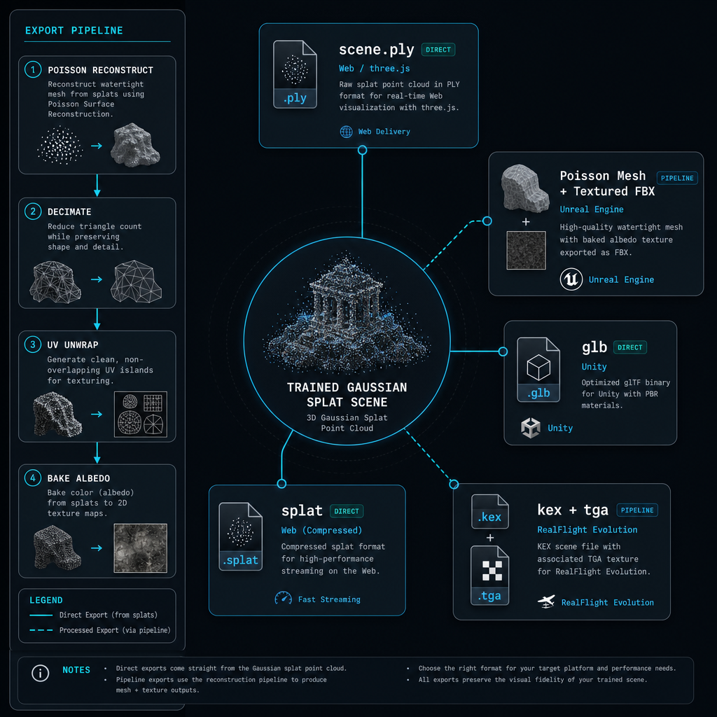
What it does
Converts the trained gaussian field into every distribution format we ship: scene.ply (raw splat — three.js, Babylon, gaussian-splats-3d, SuperSplat); scene_mesh.{glb, obj, fbx} (Poisson surface reconstruction over the splat point cloud); scene_diffuse.tga (UV-unwrapped baked albedo texture); scene_mesh.kex + .tga (RealFlight Evolution scenery, produced by running the .obj through 3ds2kex.exe).
Architecture
Sequence of independent passes: (1) splat .ply binary dump; (2) Poisson surface reconstruction on splat positions (Open3D / pymeshlab), decimate to a target face count (300 K default); (3) UV unwrap with xatlas; (4) per-texel ray into the splat field, sample colour, write into a 4096² atlas; (5) Wine + 3ds2kex.exe converts the textured .obj into RealFlight's binary scenery format (8 000-poly cap forces decimation).
Compute profile
Mostly CPU. Poisson + UV unwrap are inherently sequential. Texture bake could be parallelised but isn't. Each format is 1-5 minutes on a desktop CPU.
CUDA usage
Minimal. Texture bake could be a CUDA pass (per-texel ray-into-splat is stock GPU work) but isn't currently — it's CPU-bound, ~3 min for a 4096² atlas.
Bottlenecks
Poisson on dense (1-3 M-point) splat clouds takes minutes. Texture bake at 4096² takes minutes. UV unwrap is fastest of the three.
Adding a second machine
Each output format is independent — fan-out to workers gives ~5× speedup if you have 5 peers (one per format). Diminishing returns beyond that. Currently single-machine because the absolute time is small.
Architecture diagrams
Cross-stage system designs. Each diagram is a snapshot of how the pieces fit together — see the relevant stage above for per-step detail.
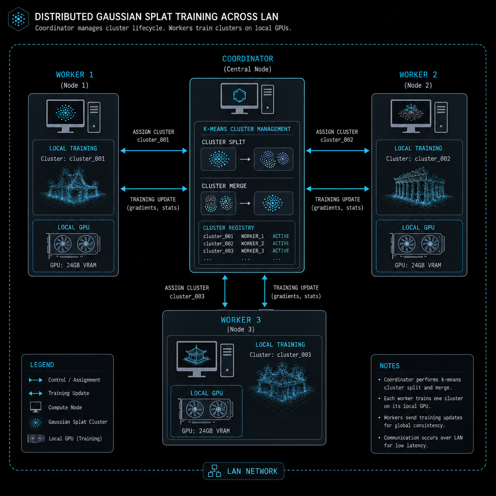
LAN farm topology (Phase C)
When two or more Splat Forge installs are on the same network, the one driving the job becomes the Coordinator. It splits the scene into clusters with k-means on the GPS positions, dispatches each cluster as a WorkOffer over a ZeroMQ ROUTER socket, and stitches the trained results back together with `colmap model_merger`. Workers DEALER-connect, train one cluster on their own GPU, tar.gz the result, and POST it back. UDP beacons on port 5557 handle peer discovery — no manual config.